In our last discussion on  the building blocks of storage we looked briefly at the expected output states for given inputs. In today’s discussion, we will take a closer look at the properties of Boolean Logic, the composition of Boolean expressions, and we will begin to see how signals propagating through the circuitry can be used to model and solve problems. To begin our discussion, let’s take a look at a generic single-output function.

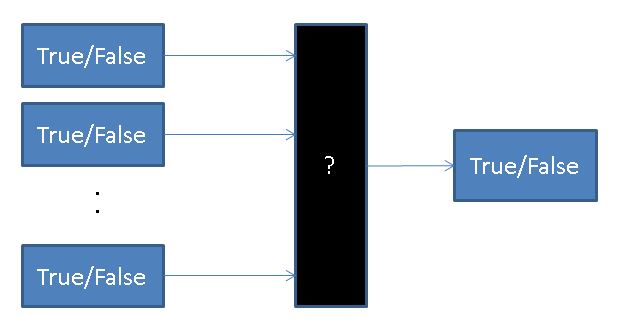
What are the possible states of this function? Below we include a table with listing the possible input and output states for 1 and 2 inputs. A table of this format is generally known as a truth table.

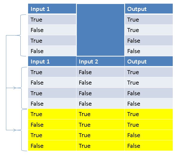
It is worth noticing, that the total number of states will double for each input added.  Generalizing to multiple inputs and outputs, the total number of possible states is 2 ^{Inputs+Outputs} ! This exponential scaling of possible states can make it impractical to perform a complete analysis on any logical process with a degree of complexity. Circuitry and software validation actually have many process similarities including mocks, simulations, and piece-wise testing!

Now that we better understand the possible states for a given logical system, we can begin to formalize our definitions of Boolean Logic. Boolean Logic serves as the bridge between the analog and digital. At its core, a computer is a series of connected circuits and storage cells. Structuring these components in certain configurations, it is possible to simulate any Logical Expression. And by chaining these Logical Expressions, we can model and work to solve any solvable problem. In Boolean Logic, there are 3 core operations.

1. NOT – Inverse of the input (true if input is false, false if input is true)
2. AND – true if all inputs are true
3. OR    – true if any input is true

By combining these operations, it becomes possible to define more complex operations. Consider the following example:

Here we see how with the addition of an AND filter in front of 2 black-box expressions, we can conditionally choose to execute one of them. Expressions similar to the above lay the foundation for reading from and writing to memory and branch selection.

Discussion:

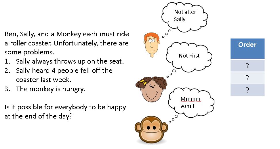
In this section, we discussed an overview of Boolean Logic and laid the foundation for a bridge between hardware and software. Above we included a link referencing the “halting problem” in computing as an example of an unsolvable problem. For consideration, it may be fun to look briefly at one problem in particular which ties directly into this section. The Boolean Satisfiability Problem. First let’s consider a scenario.

The Boolean Satisfiability Problem can be summarized as follows:

Given a Boolean Expression ƒ (Inputs), where Inputs is an Array of fixed value Boolean (true or false), return true if there is some Inputs which will invariably yield true on output.

True Example:  ƒ (I0, I1) = I0 AND I1  -> true when I0 and I1 are true

False Example: f(I0) = I0 AND (NOT I0) -> will never be true

At first, the satisfiability problem may seem distinct from our example. Let’s rewrite this in a way which better fits.

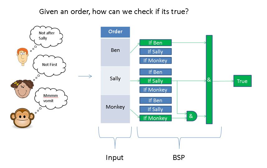
This problem and extensions of it have broad uses across computing ranging from circuit reduction to logistics problem solving. From a software front, BSP validation may act as a gatekeeper to more time-expensive logic such as only calculating an optimal solution if one exists. Amazing how such a variety of problems can be broken down to the same core issue!